Appendix A: Formulas
Updated: v2026.02.15
This appendix collects the key mathematical formulas that govern Aurora C# mechanics. Understanding these calculations helps with ship design optimization, fleet planning, and economic development.
Organization: Formulas are grouped by game phase – ship design, detection, combat, economy, and population – with related formulas kept together for easy reference.
Contents
Updated: v2026.02.15
- Appendix A: Formulas
A.1 Ship Design Formulas
Updated: v2026.02.15
Formulas used during ship design to calculate performance characteristics. For detailed ship design context, see Section 8.3 Engines.
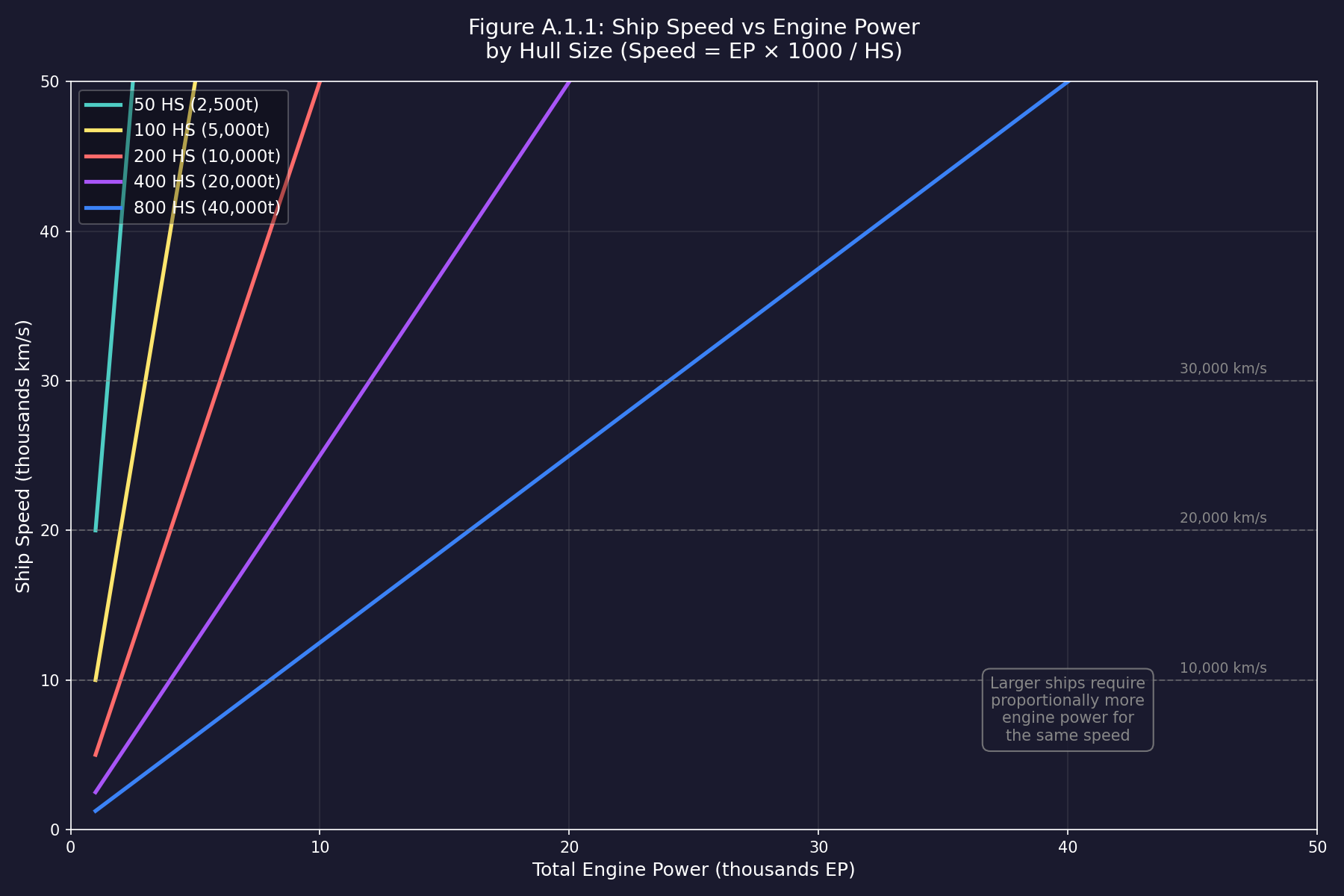
A.1.1 Ship Speed
The fundamental speed formula for any vessel \hyperlink{ref-A-1}{[A-1]}:
Speed (km/s) = Total_Engine_Power * 1000 / Ship_Size_HS
Or equivalently (since 1 HS = 50 tons) \hyperlink{ref-A-2}{[A-2]}:
Speed (km/s) = Total_Engine_Power * 50000 / Ship_Mass_tons
Where:
- Total_Engine_Power = Number_of_Engines x Engine_Power_per_Unit (in EP)
- Ship_Size_HS = Total ship size in Hull Spaces
- Ship_Mass_tons = Ship_Size_HS x 50
Example: A 200 HS ship (10,000 tons) with two engines producing 2,500 EP each:
Speed = (2 x 2500) * 1000 / 200 = 25,000 km/s
Speed = 5000 * 50000 / 10000 = 25,000 km/s (equivalent)
A.1.2 Engine Power
The actual speed depends on your engine technology. Engine power is calculated as:
Engine_Power = Engine_Size (HS) x Power_per_HS x Boost_Modifier
Where \hyperlink{ref-A-3}{[A-3]}:
- Power_per_HS is determined by engine technology research (starts at 5 with Nuclear Radioisotope Engine, increases with tech up to 100)
- Boost_Modifier ranges from 0.5x to 3.0x (higher boost = more power but reduced fuel efficiency)
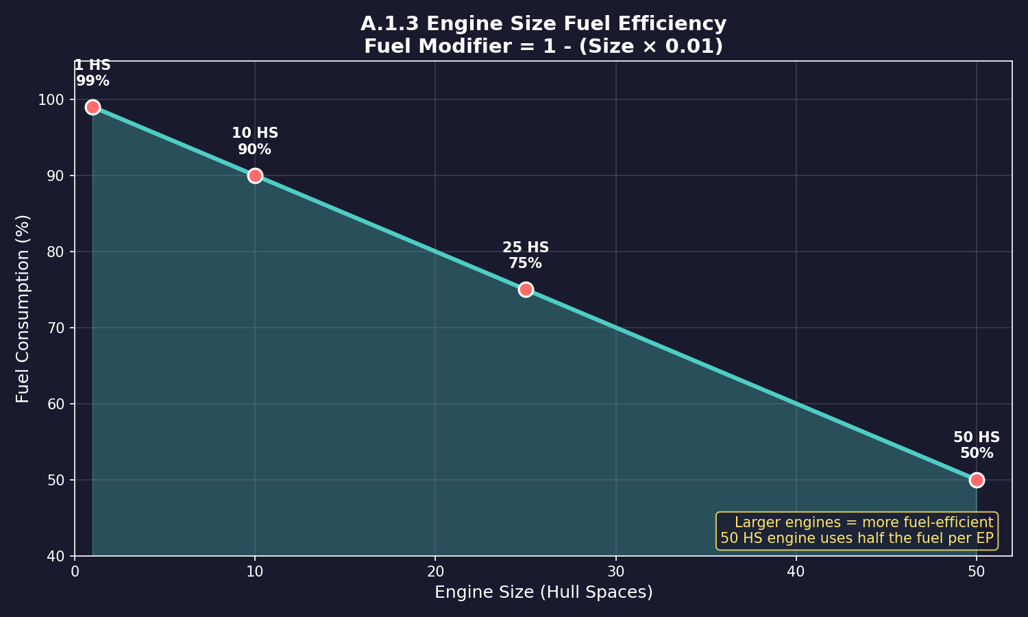
A.1.3 Engine Size-Based Fuel Consumption
In C# Aurora, engine fuel efficiency improves with engine size following a square root relationship \hyperlink{ref-A-10}{[A-10]}:
Fuel_Consumption_Modifier = SQRT(10 / Engine_Size_HS)
(unverified — #1215) — This SQRT formula replaced the linear model (1 - Engine_Size_HS * 0.01) from VB6 Aurora. The exact formula cannot be isolated from the database because fuel consumption values in FCT_ShipDesignComponents combine multiple factors (engine size, fuel consumption tech, and boost). Issue #1215 tracks full verification.
Where:
- Engine_Size_HS = Engine size in Hull Spaces
This creates efficiency advantages for larger engines:
| Engine Size (HS) | Fuel Consumption Modifier | Effect |
|---|---|---|
| 1 | 3.16 | Penalty for very small engines |
| 10 | 1.00 | Baseline (no modifier) |
| 25 | 0.63 | 37% more fuel-efficient |
| 50 | 0.45 | 55% more fuel-efficient |
Example: A 25 HS engine has fuel consumption modifier of SQRT(10/25) = 0.63, meaning it uses only 63% of the fuel per unit of power compared to a 10 HS engine.
For detailed engine design context including fuel consumption, see Section 8.3.5 Fuel Consumption.
A.1.4 Fuel Consumption Rate
Fuel_per_Hour = Total_Engine_Power x Fuel_Consumption_Rate x Boost_Penalty
Where:
- Fuel_Consumption_Rate is determined by fuel consumption technology (base 1.0, reduced by research)
- Boost_Penalty = (4 ^ Boost_Modifier) / 4, where Boost_Modifier is the power multiplier (1.0 for no boost, 1.5 for +50% boost, 2.0 for +100% boost) \hyperlink{ref-A-11}{[A-11]}. This matches the AdditionalInfo values from FCT_TechSystem TechTypeID=42. At no boost (1.0): (4^1.0)/4 = 1.0, confirming the correct baseline.
A.1.5 Range Calculation
Range (km) = Fuel_Capacity / Fuel_per_Hour x 3600 x Speed
Or equivalently:
Range (billion km) = Fuel_Capacity / (Fuel_per_Hour x 1000000)
A.1.6 Shield Strength and Regeneration
Shield_Strength = Strength_Tech x Size_HS x sqrt(Size_HS / 10)  (for generators > 1 HS)
Recharge_per_5sec = Regeneration_Tech_Level x Generator_Size_HS
Shield_EM_Signature = Shield_Strength x 3
\hyperlink{ref-A-5}{[A-5]}
Shields begin at zero when first activated and must recharge to full strength. Regeneration is continuous during combat. The strength formula’s square root scaling means larger generators provide disproportionately more shielding per HS, but recharge at the same rate per HS regardless of size.
The regeneration structure (proportional to Generator_Size_HS, not Total_Shield_Strength) is verified against the database schema – FCT_ShipDesignComponents shows regeneration values scaling with generator size. The exact coefficient/multiplier in the formula is (unverified) and may vary by implementation. See also Section D.5.3 Shield Types, which uses an incorrect formula based on Total_Shield_Strength rather than Generator_Size_HS.
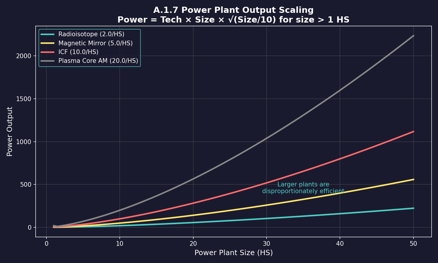
A.1.7 Power Plant Output
Power_Output = Power_Tech x Size_HS x sqrt(Size_HS)
Boosted_Output = Power_Output x Boost_Multiplier
\hyperlink{ref-A-20}{[A-20]}
This formula applies to all power plant sizes (there is no special case for small generators). Note that power plants use sqrt(Size) scaling, which is different from the sqrt(Size/10) scaling used by shields (see A.1.6). Power plants benefit more aggressively from size increases than shields do.
Explosion chance when hit is set per boost technology level (not a simple formula) \hyperlink{ref-A-4}{[A-4]}:
| Boost | Multiplier | Explosion Chance |
|---|---|---|
| None | x1.0 | 5% |
| +10% | x1.1 | 7% |
| +20% | x1.2 | 10% |
| +30% | x1.3 | 15% |
| +40% | x1.4 | 20% |
| +60% | x1.6 | 30% |
| +80% | x1.8 | 40% |
| +100% | x2.0 | 50% |
Larger power plants are more space-efficient due to the square root scaling — a 10 HS power plant produces approximately 3.16x more power per HS than a 1 HS unit.
A.1.8 Engineering Spaces
MSP_Stored = floor(12.5 x Ship_Build_Cost_BP x Engineering_Tons / Total_Ship_Tons)
AFR_Without_Engineering = 0.2 x Ship_Tonnage
AFR_With_Engineering = (0.04 / Engineering_Tonnage_Percent) x Ship_Tonnage
The factor 0.2 is a BaseFailureChance game parameter, not a direct probability percentage. Verified against FCT_ShipClass.BaseFailureChance for ships without engineering spaces (e.g., Niobe class at 984 tons yields BaseFailureChance = 196.8, matching 0.2 x 984). The interpretation of these values as annual failure probabilities is (unverified) – the raw formula produces the BaseFailureChance field value, but how the game converts this to actual component failure events during gameplay is embedded in game logic.
A.1.9 Tractor Beam Towing Speed
When a tug tows another vessel, its speed is reduced proportionally to the mass ratio:
Towing_Speed = Normal_Tug_Speed * (Tug_Mass / (Tug_Mass + Towed_Mass))
Where:
- Normal_Tug_Speed = The tug’s speed when not towing (km/s)
- Tug_Mass = The tug’s tonnage
- Towed_Mass = The towed vessel’s tonnage
Example: A 10,000-ton tug with normal speed 2,000 km/s towing a 90,000-ton ship:
Tug proportion = 10,000 / (10,000 + 90,000) = 0.10
Towing speed = 2,000 * 0.10 = 200 km/s
Heavier tugs maintain better towing speeds. The return trip (without towed vessel) is at full tug speed.
A.2 Missile Design Formulas
Updated: v2026.02.15
Formulas for missile performance calculations. See Section 12.3 Missiles for tactical context.
A.2.1 Missile Speed
Missile_Speed (km/s) = Missile_Engine_Power / Missile_Mass
Missile engines are typically much more powerful per unit mass than ship engines but have limited fuel duration:
Missile_Endurance (seconds) = Missile_Fuel / Missile_Fuel_Consumption
Missile_Range (km) = Missile_Speed x Missile_Endurance
A.2.2 High-Boost Missile Penalty
For missiles using boost exceeding racial maximum boost technology, an additional multiplier applies:
High_Boost_Modifier = (((Boost_Used - Max_Boost_Tech) / Max_Boost_Tech) * 4) + 1
This creates a linear multiplier from 1x to 5x for high-boost missiles.
A.3 Detection Formulas
Updated: v2026.02.15
Formulas governing sensor detection and electronic warfare. For detailed sensor design and usage, see Section 11.1 Thermal and EM Signatures.
A.3.1 Thermal Signature
A ship’s thermal signature is primarily determined by its engines:
Thermal_Signature = Total_Engine_Power / Thermal_Reduction_Modifier
A.3.2 Passive Sensor Detection (Thermal)
Detection_Range (km) = sqrt(Sensor_Sensitivity x Target_Thermal_Signature) x 250000
\hyperlink{ref-A-12}{[A-12]}
Where:
- Sensor_Sensitivity = Sensor_Size (HS) x Sensitivity_Tech_Level
- Target_Thermal_Signature = Total_Engine_Power / Thermal_Reduction_Tech
A.3.3 Passive Sensor Detection (EM)
Detection_Range (km) = sqrt(Sensor_Sensitivity x Target_EM_Signature) x 250000
\hyperlink{ref-A-12}{[A-12]}
Where:
- Target_EM_Signature is generated by active sensors, shields, and certain other components when active
Ships with no active emissions (shields off, active sensors off) have EM signature of 0 and are invisible to EM sensors.
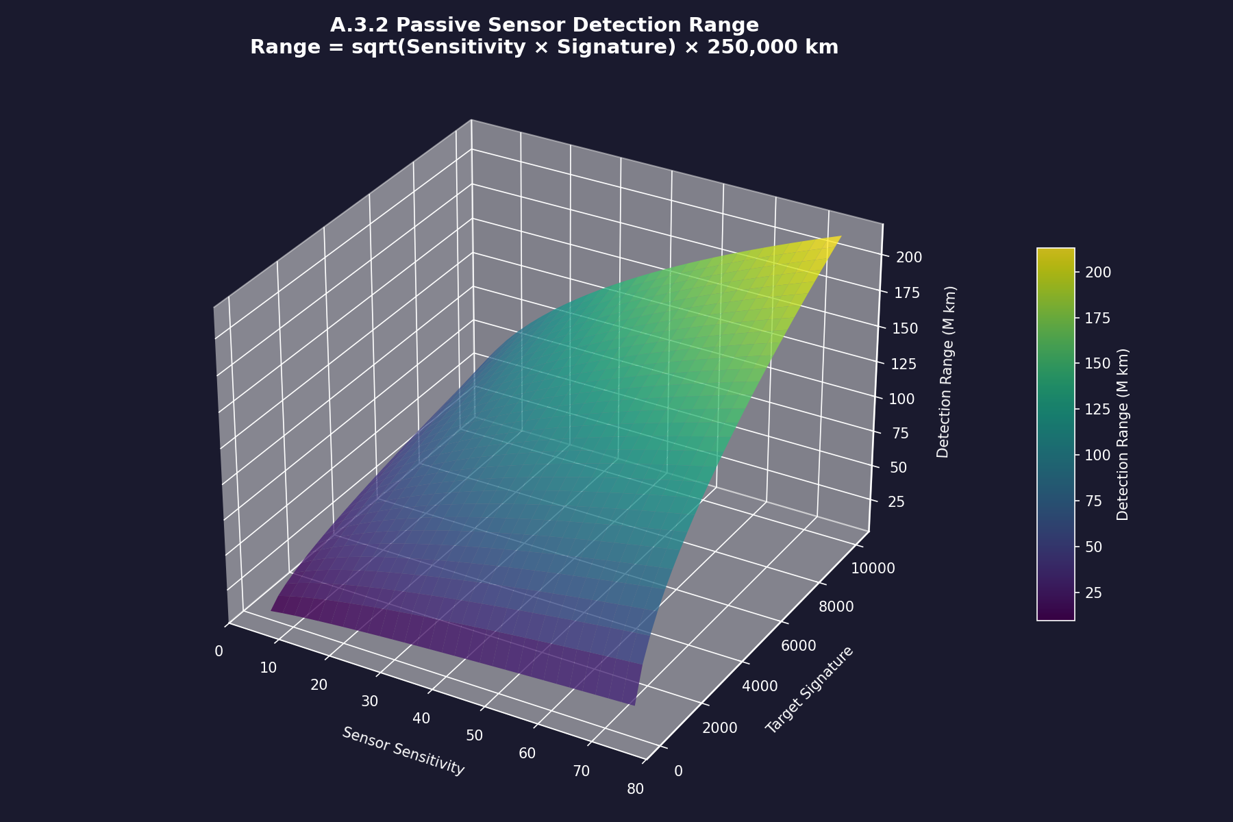
Figure A.3.2 visualizes the detection formula as a 3D surface. The square-root relationship means doubling sensor sensitivity or target signature does NOT double detection range – it increases range by only ~41%. Significant detection improvements require advances in both sensor technology and finding high-signature targets.
A.3.4 Active Sensor Detection
The game uses the following formula to calculate active sensor detection range \hyperlink{ref-A-16}{[A-16]}:
Detection_Range (km) = sqrt((Active_Strength x HS x EM_Sensitivity x Resolution^(2/3)) / PI) x 1000000
Where:
- Active_Strength = Active Grav Sensor Strength technology level (starts at 10)
- HS = Sensor size in hull spaces
- EM_Sensitivity = EM Sensor Sensitivity technology level (starts at 5)
- Resolution = Sensor resolution setting (in HS)
- PI = 3.14159…
Note: Earlier versions of this manual contained incorrect simplified forms of this formula with different multipliers (250,000 km and 10,000 km). These have been corrected. The SQRT formula in this section and in Section A.3.5 (Missile Fire Control Range) is the verified formula used throughout the manual.
Note: Some community resources use a simplified approximation:
sqrt(Sensor_Strength x Target_Cross_Section) x 250,000 km, where Sensor_Strength = Size x Resolution x Active_Tech. This approximation omits the EM Sensitivity factor and uses a different constant (250,000 vs 1,000,000), so it does not produce the same results as the full formula. The full formula above is verified against the game database and should be used for accurate calculations.
A sensor designed for resolution-100 detects 5000-ton ships at full range. Smaller ships are detected at reduced range:
Effective_Range = Base_Range x (Actual_Ship_HS / Sensor_Resolution)^(1/3)
\hyperlink{ref-A-12}{[A-12]}
Example: A sensor with 100M km range at resolution-100 detecting a resolution-20 ship:
Effective_Range = 100M x (20/100)^(1/3) = 100M x 0.585 = 58.5M km
A.3.5 Missile Fire Control Range
Missile fire controls are active sensors, so their range uses the same active sensor range formula (see Section 12.1.2 Missile Fire Controls):
MFC_Range (km) = SQRT((Active_Strength x HS x EM_Sensitivity x Resolution^(2/3)) / PI) x 1,000,000
\hyperlink{ref-A-19}{[A-19]}
Where:
- Active_Strength = Active Grav Sensor Strength technology level
- HS = Fire control sensor size in hull spaces
- EM_Sensitivity = EM Sensor Sensitivity technology level
- Resolution = Sensor resolution setting (in HS)
- PI = 3.14159…
The fire control range limits the maximum engagement distance for missiles. Missiles beyond their fire control’s range lose guidance.
A.3.6 Cloaking Effect on Detection
Effective_Signature = Actual_Signature x (1 - Cloak_Percentage/100)
A 60% cloak reduces all signatures to 40% of their actual value, reducing detection range proportionally.
A.3.7 Electronic Warfare Systems
Aurora features three distinct electronic warfare systems, each affecting different combat phases:
| System | Target | Effect | Design Placement |
|---|---|---|---|
| Sensor Jammer (SJ) | Enemy active sensors | Reduces active sensor range | Ship component |
| Fire Control Jammer (FCJ) | Enemy beam weapon accuracy | Reduces beam hit chance | Ship component |
| Missile FC Jammer (MFJ) | Missile guidance systems | Reduces missile PD accuracy | Missile component |
Note: Each jammer type is countered by a corresponding ECCM system. Net effectiveness depends on the difference between jammer level and opposing ECCM level.
Sensor Jammer Effect:
Effective_Sensor_Range = Base_Range x (1 - (Target_SJ_Level - Sensor_ECCM_Level) x 0.1)
Where:
- Minimum effective range is 0 (complete sensor denial at 10+ net advantage) \hyperlink{ref-A-17}{[A-17]}
- If ECCM >= SJ, no reduction applies
Fire Control Jammer Effect (ECM):
ECM_Mod = max(0, 1 - (Target_ECM - FC_ECCM) x 0.1)
Applied as a multiplier to beam weapon hit chance. See Beam Weapon To-Hit for the complete formula.
Missile FC Jammer Effect:
ECM_ECCM_Mod = 1 - ((Missile_FC_Jammer_Level - CIWS_ECCM_Level) * 0.1)
Minimum 0 (complete jamming). Applied to point defense accuracy against missiles. See Point Defense Accuracy for the complete formula.
A.4 Combat Formulas
Updated: v2026.02.15
Formulas governing weapons, damage, and defensive systems. For tactical combat details, see Section 12.1 Fire Controls.
A.4.1 Time to Destination
Time (seconds) = Distance (km) / Speed (km/s)
For jump point transits, add the transit time (typically instantaneous for military jump drives, or 5 minutes for commercial jump drives including squadron transit).
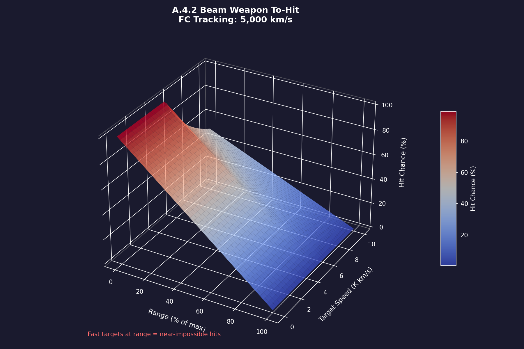
A.4.2 Beam Weapon To-Hit
Base_Chance = (1 - Range/Max_Range) x 100%
Tracking_Mod = min(1.0, Tracking_Speed / Target_Speed)
ECM_Mod = max(0, 1 - (Target_ECM - FC_ECCM) x 0.1)
Final_Chance = Base_Chance x Tracking_Mod x ECM_Mod
Note: The 0.1 coefficient (10% reduction per net ECM level) is consistent with the database’s integer ECM levels (0-10) and ECCM levels (0-10), but the exact coefficient is embedded in game combat logic. The formula structure is confirmed by community testing.
Example: Laser at 50% of max range, tracking 5000 km/s vs target at 4000 km/s, target ECM-2 vs FC ECCM-1:
Base = (1 - 0.5) x 100 = 50%
Tracking = min(1.0, 5000/4000) = 1.0
ECM = max(0, 1 - (2-1) x 0.1) = 0.9
Final = 50% x 1.0 x 0.9 = 45%
A.4.3 Beam Weapon Damage
Beam weapon damage is governed by two mechanics: damage falloff with range and damage gradient (armor column spread). See Section 12.2.2 for full tactical discussion.
Damage Falloff (Range-Dependent)
Only lasers suffer damage falloff. The formula is a linear reduction:
Damage_at_Range = Base_Damage * (1 - Range / Max_Range)
At point-blank (Range = 0), full damage is dealt. At max range, damage approaches the minimum (1 point). Damage steps down in discrete range increments (typically 10,000 km brackets).
Weapons with damage gradient of 1 deal full base damage at any range within their maximum envelope—no falloff applies.
Damage Falloff by Weapon Type:
| Weapon Type | Damage Gradient | Range Falloff | Notes |
|---|---|---|---|
| Lasers | 3-4 | Linear (formula above) | Primary weapon affected by falloff |
| Particle Beams | 2 | None (full damage at all ranges) | Steep penetration profile |
| Plasma Carronades | 1 | None (full damage at all ranges) | Short max range, half-size |
| Railguns | 2 | None (full damage at all ranges) | Multiple shots per salvo |
| Meson Cannons | 1 | None | Always 1 damage; bypasses armor/shields |
| Microwaves (HPM) | 1 | None (full damage at all ranges) | Targets electronics after shields down |
| Gauss Cannons | 1 | None | 1 damage per shot, high rate of fire |
Damage Gradient (Armor Column Spread)
The gradient value determines how many adjacent armor columns receive damage per hit:
Damage_per_Column ≈ Total_Damage / Gradient_Value
- Gradient 1: All damage in 1 column (focused penetration)
- Gradient 3: Damage spread across 3 columns (standard lasers)
- Gradient 4: Damage spread across 4 columns (large-caliber lasers)
Combined Effect (Laser at Range):
For a laser with damage falloff AND gradient spread, both apply:
Per_Column_Damage = (Base_Damage * (1 - Range / Max_Range)) / Gradient_Value
Armor_Penetration = Per_Column_Damage (must exceed armor depth to reach internals)
Example: A 20-damage laser (gradient 3) firing at 50% of max range:
Total_Damage = 20 * (1 - 0.5) = 10
Per_Column = 10 / 3 ≈ 3.3 → each of 3 columns takes ~3 damage
Armor_Penetration = ~3 layers per column
Compare with a particle beam (gradient 2) with 10 base damage at the same range:
Total_Damage = 10 (no falloff)
Per_Column = 10 / 2 = 5
Armor_Penetration = 5 layers across 2 columns
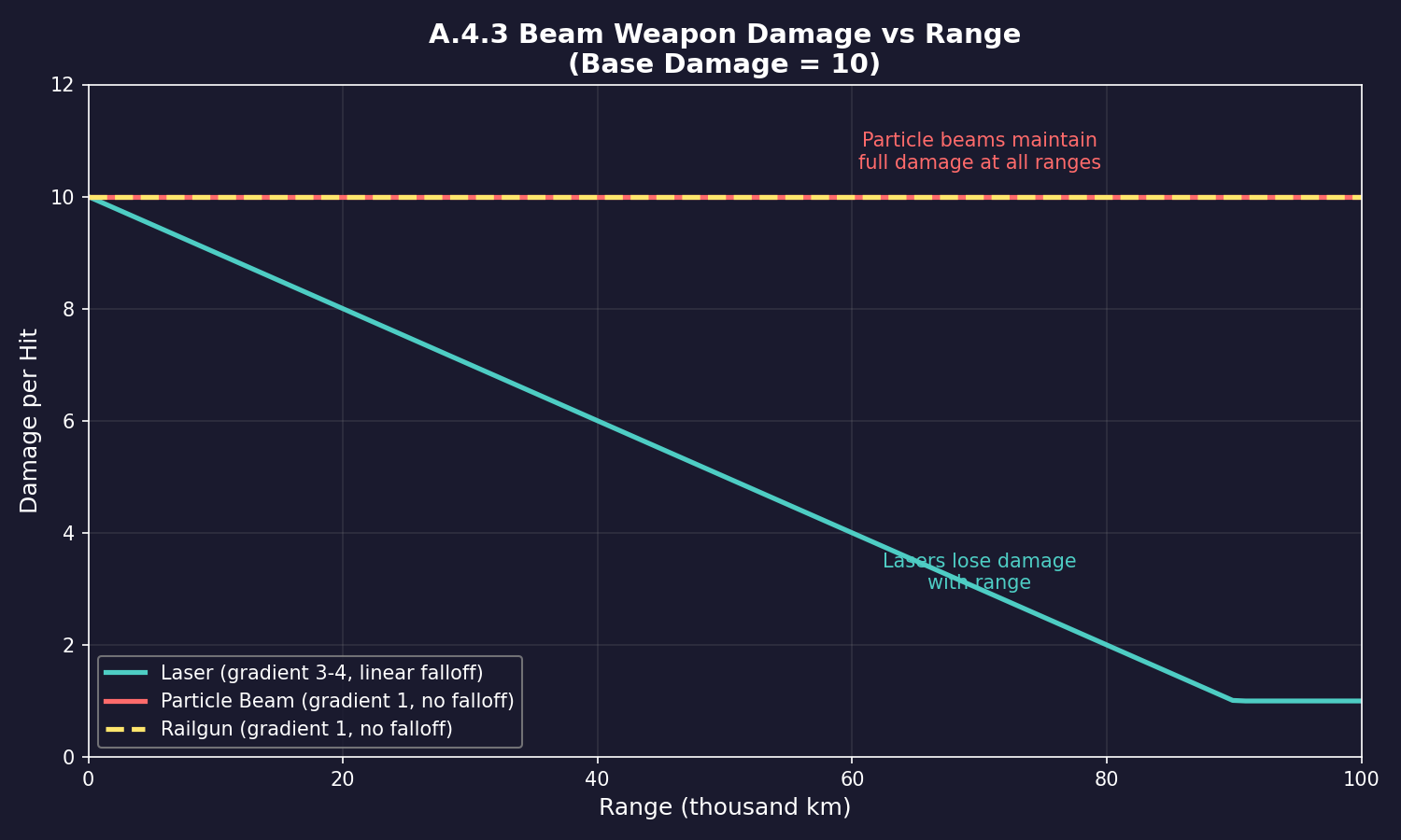
Figure A.4.3 compares damage output across range for the three primary beam weapon types. Lasers (cyan) suffer linear damage falloff, making them less effective at long range. Particle beams (red) and railguns (yellow) maintain full damage at all ranges within their envelope, making them superior for consistent damage at range despite lower base damage values.
A.4.4 Armor Damage
Armor_Columns = Ship_Width (proportional to tonnage)
Damage_per_Column = Weapon_Damage (applied to random column)
Penetration = Damage_Applied > Remaining_Armor_at_Column
Armor column count scales with ship size:
Num_Columns = Ship_Tonnage / Column_Factor
A.4.5 Internal Damage
When armor at a column is breached:
Component_Hit_Chance = Component_HS / Total_Internal_HS
Damage_to_Component = 1 HTK per hit
Component_Destroyed when Current_HTK = 0
A.4.6 Shock Damage
Shock_Chance = Armor_Damage / Ship_Size_HS  (minimum 5% threshold; below = ignored)
Shock_Amount = Random(0 to floor(Armor_Damage x 0.20))
Shields completely negate shock damage. Only damage applied to armor triggers the shock check.
A.4.7 Magazine Explosion
Explosion_Damage = Sum(All_Missile_Warhead_Strengths_in_Magazine)
Applied to the host ship first, excess may damage nearby vessels within blast radius.
A.4.8 Missile Hit Chance (Speed Ratio System)
Base_Hit_Chance = 0.1 * (Missile_Speed / Target_Speed)
Where:
- Missile_Speed = The missile’s designed speed (km/s)
- Target_Speed = The target’s current speed (km/s)
Example: A 30,000 km/s missile against a 5,000 km/s target:
Base Hit Chance = 0.1 * (30,000 / 5,000) = 0.6 = 60%
Active Terminal Guidance (0.25 MSP component) provides an accuracy bonus from +15% to +60% based on technology level, applied as a multiplier to the base hit chance \hyperlink{ref-A-13}{[A-13]}.
Key implications:
- Against stationary targets, hit chance is effectively 100% (infinite speed ratio)
- Faster missiles are more accurate; very fast targets require proportionally faster missiles
- Multiple warheads provide additional independent hit rolls
A.4.9 Missile Point Defense
For each PD weapon firing at incoming missiles:
Intercept_Chance = (1 - Range/Max_Range) x Tracking_Mod x 100%
Where Tracking_Mod for PD against missiles:
Tracking_Mod = min(1.0, PD_Tracking / Missile_Speed)
CIWS (Close-In Weapon Systems) fire at range 0 (final defense), making their base chance very high, but they must track the missile’s speed.
A.4.10 Point Defense Accuracy (CIWS Effectiveness)
The complete PD accuracy formula for CIWS and beam weapons in point defense mode:
Hit_Probability = Base_Tracking_Mod * Crew_Training * ECM_ECCM_Mod * CIC_Bonus * Tactical_Bonus * Gauss_Size_Mod * Range_Mod
Where:
- Base_Tracking_Mod = min(1.0, FC_Tracking_Speed / Missile_Speed)
- Crew_Training = Fractional modifier based on crew training level (1.0 at 100% training)
- ECM_ECCM_Mod = 1 - ((Missile_FC_Jammer_Level - CIWS_ECCM_Level) * 0.1), minimum 0
- CIC_Bonus = Commander’s Combat Information Center skill bonus
- Tactical_Bonus = Commander’s Tactical skill bonus
- Gauss_Size_Mod = Per-shot accuracy modifier for gauss cannons below racial standard size
- Range_Mod = 1.0 within 10,000 km (Point Blank modes); decreases with distance beyond 10,000 km
Expected Kills per Tick:
Expected_Kills = Shots_per_Tick * Hit_Probability
Example: A triple-turret gauss cannon with rate-of-fire 4 technology fires 12 shots per burst. Against missiles at 80% tracking (FC tracks faster than missile) with no ECM:
Expected kills = 12 * 0.8 = 9.6 missiles per 5-second cycle
A.5 Production Formulas
Updated: v2026.02.15
Formulas for economic output and industrial production. For colony production management, see Section 6.3 Construction.
A.5.1 Construction Factory Output
Annual_BP = Num_Factories x BP_per_Factory x (1 + Governor_Production_Bonus)
Note: The exact governor production bonus formula requires verification. Section 18.1 indicates the actual mechanic is a percentage-based Production bonus, not a flat multiplier. (unverified — #1246)
Standard BP per factory = 10/year (increased by Construction Rate technology) \hyperlink{ref-A-6}{[A-6]}:
| Technology Level | BP per Factory | Research Cost (RP) |
|---|---|---|
| Base | 10 | – |
| 1 | 12 | 3,000 |
| 2 | 14 | 5,000 |
| 3 | 16 | 10,000 |
| 4 | 20 | 20,000 |
| 5 | 25 | 40,000 |
| 6 | 30 | 80,000 |
| 7 | 36 | 150,000 |
| 8 | 42 | 300,000 |
| 9 | 50 | 600,000 |
| 10 | 60 | 1,250,000 |
| 11 | 70 | 2,500,000 |
A.5.2 Mineral Mining Output
Annual_Tons_per_Mine = Base_Production x Accessibility x Tech_Modifier
Where Base_Production = 10 tons/year per mine \hyperlink{ref-A-7}{[A-7]}. Mining technology progression:
| Technology Level | Tons/Mine/Year | Research Cost (RP) |
|---|---|---|
| Base | 10 | – |
| 1 | 12 | 3,000 |
| 2 | 14 | 5,000 |
| 3 | 16 | 10,000 |
| 4 | 20 | 20,000 |
| 5 | 25 | 40,000 |
| 6 | 30 | 80,000 |
| 7 | 36 | 150,000 |
| 8 | 42 | 300,000 |
| 9 | 50 | 600,000 |
| 10 | 60 | 1,250,000 |
| 11 | 70 | 2,500,000 |
A.5.3 Fuel Refinery Output
Fuel_per_Year = Num_Refineries x Base_Output_per_Refinery (litres)
Base refinery output is 40,000 litres/year \hyperlink{ref-A-8}{[A-8]}. Refinery technology progression:
| Technology Level | Output (litres/year) | Research Cost (RP) |
|---|---|---|
| Base | 40,000 | – |
| 1 | 48,000 | 3,000 |
| 2 | 56,000 | 5,000 |
| 3 | 64,000 | 10,000 |
| 4 | 80,000 | 20,000 |
| 5 | 100,000 | 40,000 |
| 6 | 120,000 | 80,000 |
| 7 | 144,000 | 150,000 |
| 8 | 168,000 | 300,000 |
| 9 | 200,000 | 600,000 |
| 10 | 240,000 | 1,250,000 |
| 11 | 280,000 | 2,500,000 |
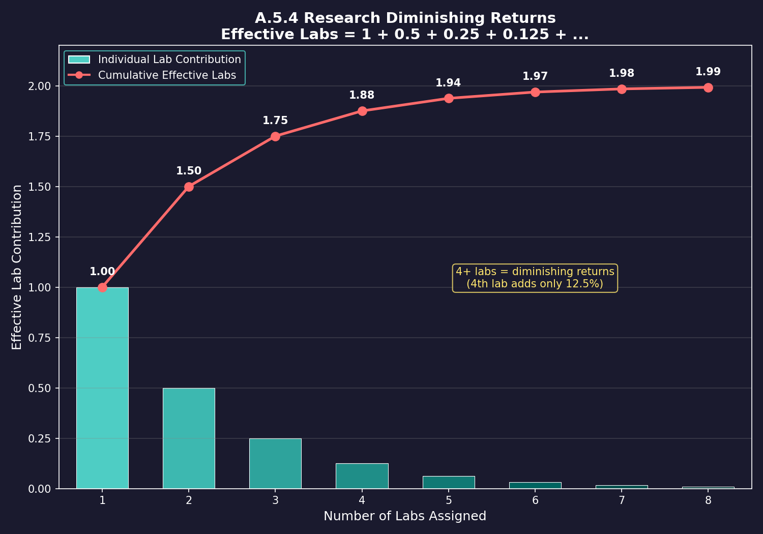
A.5.4 Research Speed
Days_to_Complete = Research_Cost / (Daily_RP_Output)
Daily_RP_Output = Sum_of_All_Labs_on_Project / 365
With diminishing returns for multiple labs \hyperlink{ref-A-15}{[A-15]}:
Effective_Labs = Lab_1 + Lab_2 x 0.5 + Lab_3 x 0.25 + Lab_4 x 0.125 + ...
RP_per_Year = Effective_Labs x RP_per_Lab x (1 + Scientist_Bonus / 100)
Where Scientist_Bonus is the percentage shown in the commander’s profile. This bonus is quadrupled when the scientist works in their specialization field.
A.5.5 Terraforming Rate
Atm_Change_per_Year = Num_Installations x Terraform_Rate x Gas_Modifier
Where:
- Terraform_Rate depends on the technology level of terraforming installations
- Gas_Modifier varies by the gas being added or removed (some gases terraform faster than others)
Terraforming rate technology progression \hyperlink{ref-A-9}{[A-9]}:
| Technology Level | Rate (atm/year) | Research Cost (RP) |
|---|---|---|
| Racial Starting Rate | 0.00025 | — |
| Terraforming Rate 1 | 0.00032 | 3,000 |
| Terraforming Rate 2 | 0.0004 | 5,000 |
| Terraforming Rate 3 | 0.00048 | 10,000 |
| Terraforming Rate 4 | 0.0006 | 20,000 |
| Terraforming Rate 5 | 0.00075 | 40,000 |
| Terraforming Rate 6 | 0.00096 | 80,000 |
| Terraforming Rate 7 | 0.0012 | 150,000 |
| Terraforming Rate 8 | 0.0015 | 300,000 |
| Terraforming Rate 9 | 0.0019 | 600,000 |
| Terraforming Rate 10 | 0.0024 | 1,200,000 |
| Terraforming Rate 11 | 0.003 | 2,500,000 |
| Terraforming Rate 12 | 0.00375 | 5,000,000 |
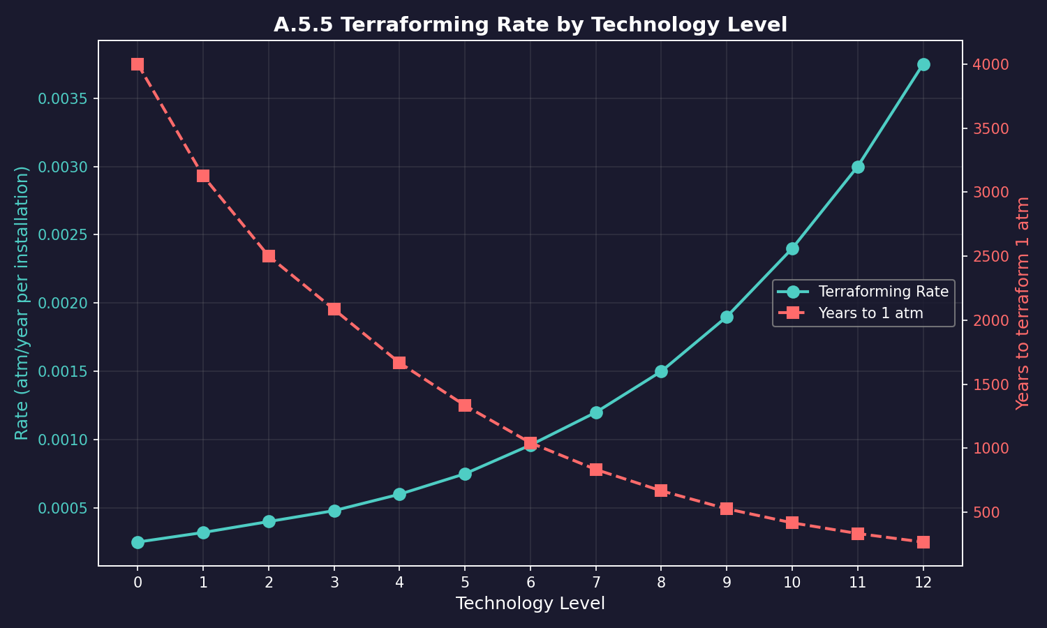
Figure A.5.5 shows the terraforming rate progression (cyan) alongside the inverse: years required to terraform 1 atmosphere with a single installation (red). Higher technology provides exponential-like acceleration – at tech level 12, terraforming is 15x faster than at base tech.
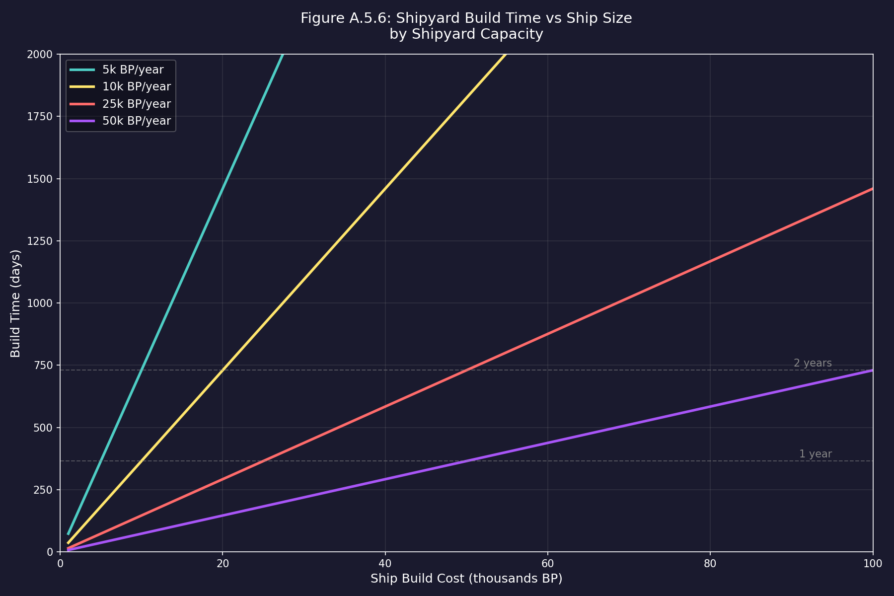
A.5.6 Shipyard Build Time
Build_Time (days) = Ship_BP_Cost / (Shipyard_Capacity / 365) / Num_Slipways
But note: a single ship can only be built in one slipway. Multiple slipways allow parallel construction of multiple ships, not faster construction of a single ship.
Retooling time when changing ship class:
Retool_Time (days) = abs(New_Ship_Tonnage - Old_Ship_Tonnage) x Retool_Factor
A.5.7 Secondary Build (20% Refit Cost Rule)
A shipyard can build any secondary class without retooling if the refit cost is below 20% of the primary class’s total build cost:
Eligible_for_Secondary_Build = (Refit_Cost < 0.20 * Primary_Class_BP_Cost)
Where:
- Refit_Cost = Build point cost to refit the primary class into the secondary class
- Primary_Class_BP_Cost = Total build point cost of the class the shipyard is currently tooled for
Example: A destroyer with 2,000 BP build cost can build secondary classes whose refit cost is under 400 BP (20% of 2,000). An escort variant swapping missile launchers for gauss cannons at 300 BP refit cost is eligible; a variant replacing engines and adding a jump drive at 800 BP is not.
This allows shipyard flexibility when designing ship families that share expensive components (engines, reactors) while varying cheaper components (cargo holds, troop bays).
A.6 Population and Colony Formulas
Updated: v2026.02.15
Formulas for population growth, habitability, and colony management. For colony management and habitability, see Section 5.1 Establishing Colonies.
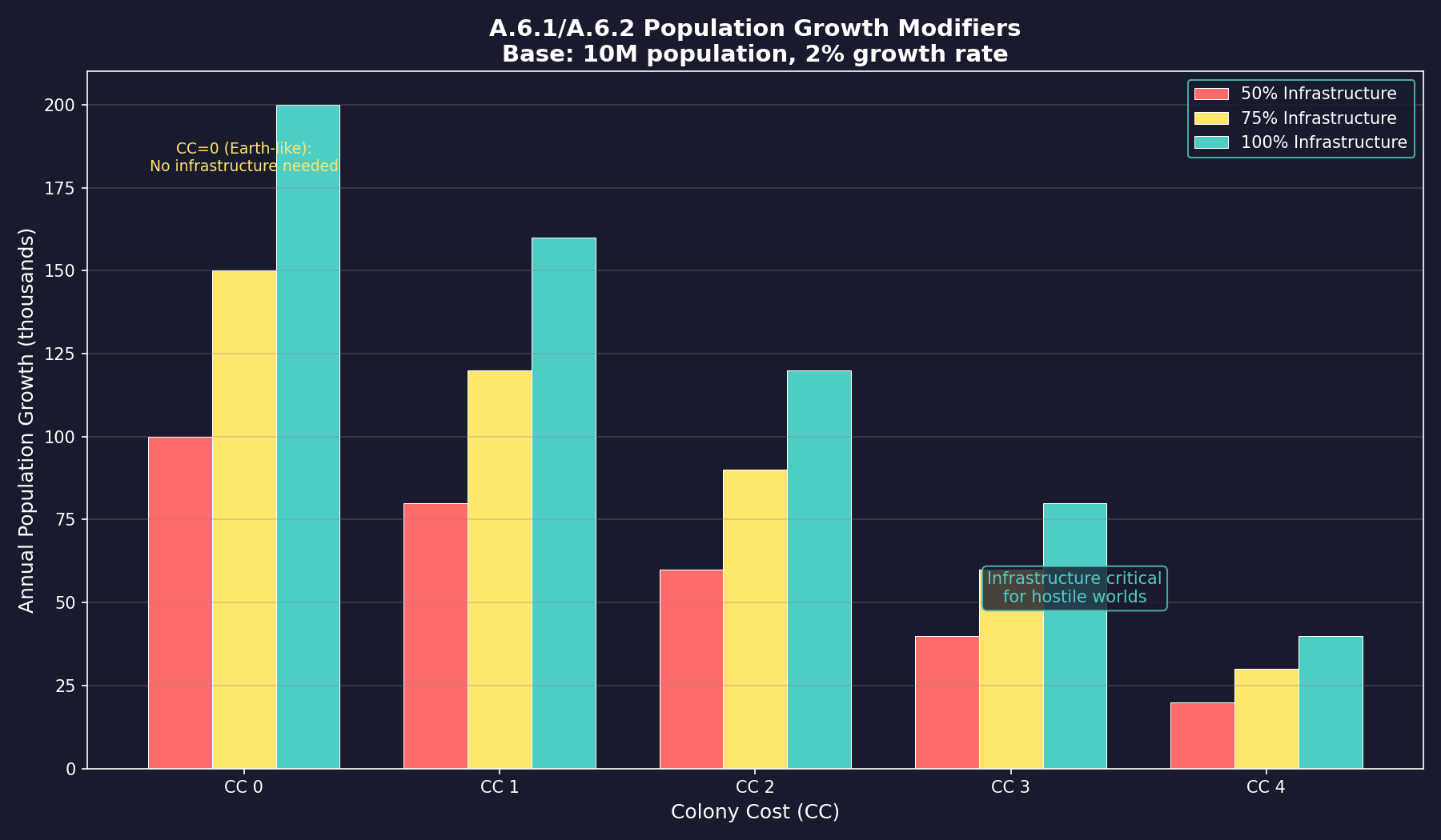
A.6.1 Base Growth Rate
Annual_Growth = Population x Growth_Rate x Habitability_Modifier x Infrastructure_Modifier
Where:
- Growth_Rate = Base racial growth rate (typically 0.02 to 0.05 or 2-5% per year)
- Habitability_Modifier = Planet’s colony cost modifier (1.0 for ideal, reduced for hostile environments)
- Infrastructure_Modifier = min(1.0, Infrastructure_Units / Required_Infrastructure)
A.6.2 Growth Rate Modifiers
| Condition | Modifier |
|---|---|
| Ideal planet (CC = 0) | 1.0x |
| Low infrastructure | Proportional reduction |
| Overcrowding | Growth reduced progressively |
| Governor bonus | 1 + (Admin_Skill x 0.05) |
| Genetic modification tech | Increases base racial growth rate |
A.6.3 Colony Cost and Habitability
Colony_Cost = Max(Environmental_Penalties)
Colony cost equals the single highest (worst) environmental penalty factor, not the sum of all factors \hyperlink{ref-A-18}{[A-18]}. Environmental penalties include:
- Temperature deviation from ideal (per degree of difference)
- Atmospheric pressure deviation
- Hostile gas presence
- Gravity deviation (minor effect)
Required_Infrastructure = Population (millions) x Colony_Cost x 100
Without sufficient infrastructure on a hostile world, excess population suffers attrition.
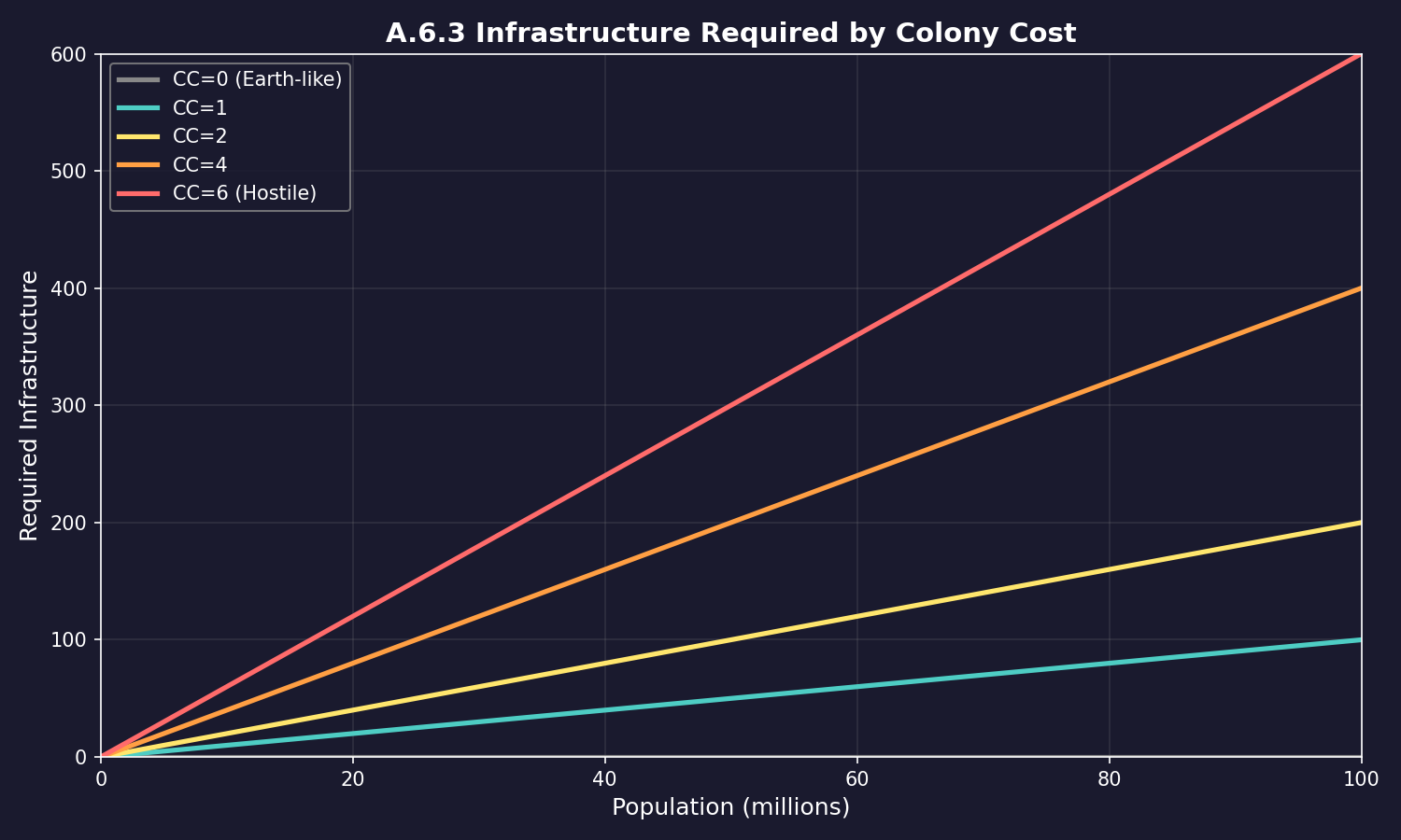
Figure A.6.3 demonstrates why extreme colony costs make expansion prohibitively expensive. A 100-million population on a CC 6.0 world requires 60,000 infrastructure units, while the same population on CC 2.0 needs only 20,000. Earth-like worlds (CC 0) require no infrastructure at all.
A.6.4 Population Capacity
Max_Supported_Population (millions) = Infrastructure / (Colony_Cost x 100)
For Earth-like worlds (colony cost = 0), no infrastructure is needed and population can grow without limit.
A.6.5 Civilian Infrastructure Production
Civilian shipping lines produce infrastructure for colonies with colony cost > 0, at no cost to the government:
Annual_Infrastructure = 2 * Population (in millions)
Where:
- Population = The colony’s population in millions
- Only colonies with Colony Cost > 0 demand and receive this production
- On low-gravity worlds, civilian production generates LG-Infrastructure at one-third the normal rate
Example: A colony of 10 million on a CC 2.0 world receives approximately 20 infrastructure units per year from civilian production alone.
This supplements but does not replace government construction, especially in early colonization stages when infrastructure needs are urgent.
A.6.6 Agriculture & Environment Workforce
A portion of the manufacturing workforce is diverted to agriculture and environmental support based on colony cost:
Agriculture_Workers_Percent = 5 + (5 x Colony_Cost)
Effective_Industrial_Workers = Total_Population x 0.60 x (1 - Agriculture_Workers_Percent / 100)
Where:
- 0.60 = Approximately 60% of total population is available as workers (remainder are children, elderly, service sector)
- Colony_Cost = The colony’s environmental cost factor (0.0 for Earth-like worlds)
Examples:
CC 0.0: Industrial Workers = Pop x 0.60 x 0.95 = Pop x 0.57
CC 2.0: Industrial Workers = Pop x 0.60 x 0.85 = Pop x 0.51
CC 4.0: Industrial Workers = Pop x 0.60 x 0.75 = Pop x 0.45
A.6.7 Migration
When multiple colonies exist, population can migrate between them based on:
- Relative habitability
- Available jobs (installations require workers)
- Overcrowding at source colony
- Automated migration policies set by the player
Migration_Rate = Base_Rate x Push_Factor x Pull_Factor
A.7 Garrison and Unrest Formulas
Updated: v2026.02.15
Formulas for occupation, garrison requirements, and population unrest. See Section 13.1 Unit Types for ground force details.
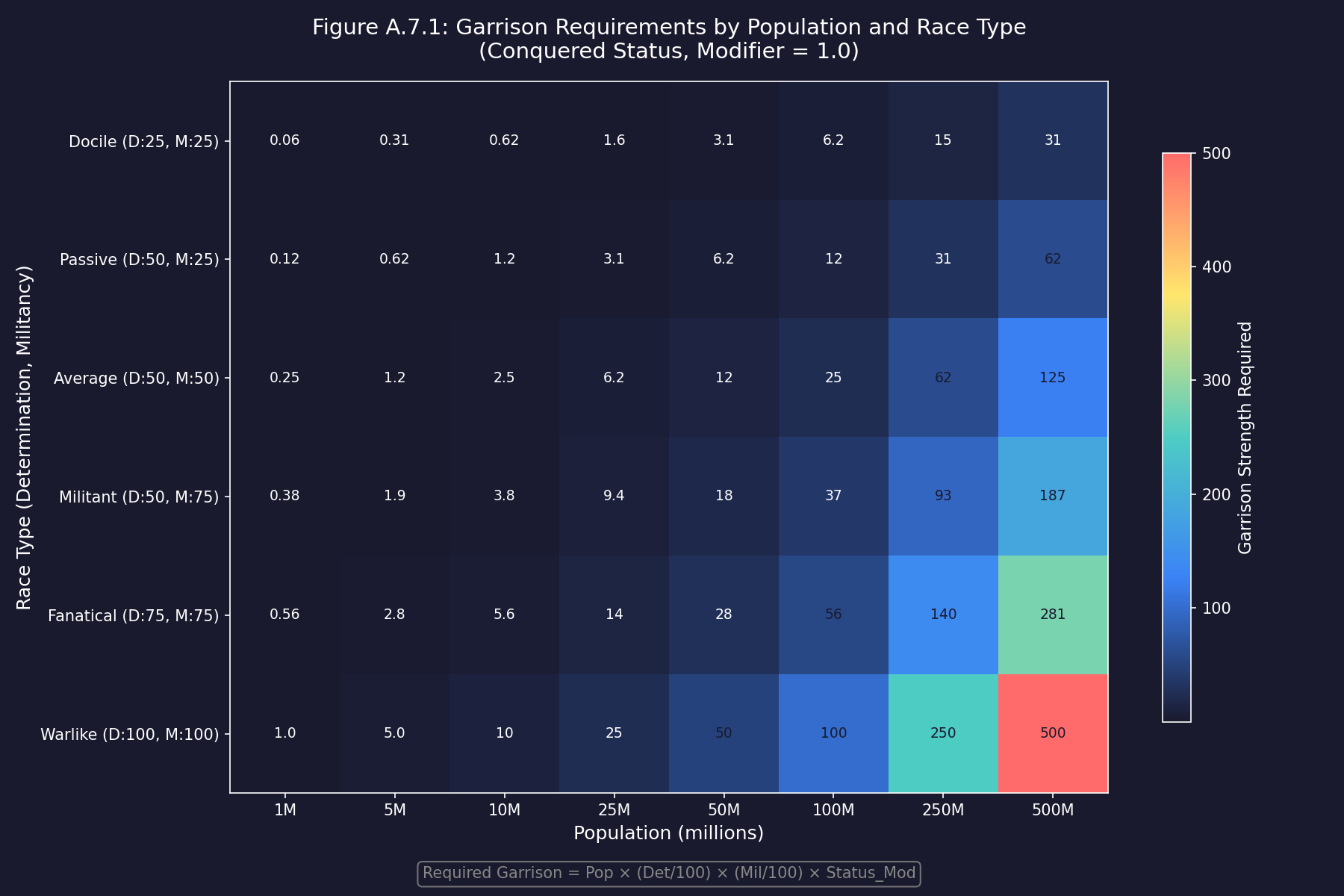
A.7.1 Required Garrison Strength
(unverified) — This formula is a simplified version that uses only two racial factors (Determination and Militancy). The more complete formula in Section A.7.3 Unrest and Stability includes Xenophobia as a third factor and applies the Political Status Modifier multiplicatively, which is more consistent with the database schema (FCT_Race includes Determination, Militancy, and Xenophobia fields). Use A.7.3 for accurate calculations.
The garrison strength required to maintain order on a colony is approximately:
Required_Garrison = Population (millions) * (Racial_Determination / 100) * (Racial_Militancy / 100)
Where:
- Population = The colony’s population in millions
- Racial_Determination = The race’s determination rating (higher = more resistant to occupation)
- Racial_Militancy = The race’s militancy rating (higher = more prone to armed resistance)
For occupied populations, a Political Status Modifier applies:
| Political Status | Modifier |
|---|---|
| Slave Colony | 1.5 |
| Conquered | 1.0 |
| Occupied | 0.75 |
| Subjugated | 0.25 |
| All Others | 0 |
A.7.2 Element Occupation Strength
Per ground unit element:
Occupation_Strength = (SQRT(Size) * Units * Morale) / 10,000
When occupation strength exceeds the requirement, the surplus functions as police strength that actively reduces unrest over time.
A.7.3 Unrest and Stability
Population unrest affects productivity. Production output (factories, research, shipbuilding) is reduced by a percentage equal to the current unrest points. At 25 unrest points, all output drops by 25%.
Effective_Production = Base_Production x (1 - Unrest_Points / 100)
Unrest Sources and Annual Point Generation:
| Source | Annual Unrest Points | Formula |
|---|---|---|
| Radiation | Radiation Level / 10 | e.g., radiation 1000 = 100 points/year |
| Overcrowding | 25 x (Missing Infrastructure / Available Infrastructure) | Baseline of 25 if no infrastructure at all |
| Insufficient Occupation Forces | 100 x (1 - Actual Strength / Required Strength) | 100 points if no forces present |
| Insufficient Local Defence | 25 x (1 - Total PPV / Required Protection) | Based on Population Protection Value |
| Forced Labour Construction | +5 per camp when built | Immediate, one-time addition |
Required Occupation Strength:
Required = Population x ((Determination + Militancy + Xenophobia) / 300) x Political Status Modifier
Required Protection (PPV):
Required = Population (millions) x (Militancy / 100) x Political Status Protection Modifier
Population Threshold: PPV requirements only apply to colonies with 10 million or more population. Smaller colonies do not generate unrest from insufficient local defence. (unverified — #874 – threshold from community sources, needs authoritative confirmation)
Ships are evaluated by Population Protection Value (hull space allocated to weapons and hangar bays). PPV is calculated system-wide — a single armed ship or PDC provides protection for all colonies in the system.
A.7.4 Unrest Reduction
Natural decline (when the cause is removed):
Fall in Unrest Points = 20 x (1 - (Determination / 100))
Military suppression (when occupation strength exceeds requirement):
Police Strength = Actual Occupation Strength - Required Occupation Strength
Reduction in Unrest = 100 x (Police Strength / Effective Population Size)
Where Effective Population Size = ((Determination + Militancy + Xenophobia) / 300) x Population Amount
Related Sections
- Section 5.1 Establishing Colonies — Population growth, colony cost, and habitability mechanics
- Section 5.2 Population — Workforce allocation and population capacity
- Section 5.4 Infrastructure — Infrastructure production and installation types
- Section 6.2 Mining — Production, mining, and refining installations
- Section 8.3 Engines — Engine, speed, and fuel consumption design parameters
- Section 8.6 Other Components — Tractor beams, power plants, and engineering spaces
- Section 9.1 Shipyards — Shipyard capacity, retooling, and secondary build rules
- Section 11.1 Thermal and EM Signatures — Sensor range and detection calculations
- Section 12.1 Fire Controls — Beam weapons, missiles, armor, and shield combat mechanics
- Section 12.3 Missiles — Missile hit chance and speed ratio system
- Section 12.4 Point Defense — CIWS effectiveness and PD accuracy formulas
- Section 13.1 Unit Types — Garrison strength and occupation mechanics
- Section 14.1 Fuel — Fuel consumption and logistics
- Appendix D: Reference Tables — Quick-reference tables for minerals, installations, and technology
References
\hypertarget{ref-A-1}{[A-1]} AuroraWiki Engine page – Speed formula: “One unit of engine power is the amount of power required to propel 50 tons (1 HS) at 1000 km/s.” Speed = Total_EP x 1000 / Ship_Size_HS.
\hypertarget{ref-A-2}{[A-2]} Aurora C# game database (AuroraDB.db v2.7.1) – 1 HS = 50 tons is a core game constant used throughout ship design.
\hypertarget{ref-A-3}{[A-3]} Aurora C# game database (AuroraDB.db v2.7.1) – FCT_TechSystem TechTypeID=40 (Engine Technology): 15 engine types from Conventional (1.0 power/HS, 500 RP) through Quantum Singularity Drive (100.0 power/HS, 5,000,000 RP). TechTypeID=130 (Max Engine Power Modifier): x1 through x3 (15,000 RP). TechTypeID=198 (Min Engine Power Modifier): x0.5 through x0.1 (30,000 RP).
\hypertarget{ref-A-4}{[A-4]} Aurora C# game database (AuroraDB.db v2.7.1) – FCT_TechSystem TechTypeID=42 (Power vs Efficiency): 8 boost levels from None (x1.0, 5% explosion, 250 RP) through +100% (x2.0, 50% explosion, 30,000 RP). Explosion percentages are discrete per-level values, not derived from a simple formula.
\hypertarget{ref-A-5}{[A-5]} Aurora C# game database (AuroraDB.db v2.7.1) – FCT_TechSystem TechTypeID=16 (Shield Type): 12 shield types from Alpha (1.0/HS, 1,000 RP) through Omega (15.0/HS, 2,000,000 RP). TechTypeID=14 (Shield Regeneration Rate): 12 levels from 1.0 (1,000 RP) through 15.0 (2,000,000 RP).
\hypertarget{ref-A-6}{[A-6]} Aurora C# game database (AuroraDB.db v2.7.1) – FCT_TechSystem TechTypeID=25 (Improved Construction Rate): 11 levels from 12 BP (3,000 RP) through 70 BP (2,500,000 RP). DIM_PlanetaryInstallation confirms base Construction Factory output of 1.0 (ConstructionValue column), representing 10 BP/year at base tech.
\hypertarget{ref-A-7}{[A-7]} Aurora C# game database (AuroraDB.db v2.7.1) – FCT_TechSystem TechTypeID=26 (Improved Mining Production): 11 levels from 12 tons (3,000 RP) through 70 tons (2,500,000 RP). DIM_PlanetaryInstallation confirms Mine base MiningProductionValue of 1.0 (10 tons/year).
\hypertarget{ref-A-8}{[A-8]} Aurora C# game database (AuroraDB.db v2.7.1) – FCT_TechSystem TechTypeID=32 (Improved Fuel Production): 11 levels from 48,000 litres (3,000 RP) through 280,000 litres (2,500,000 RP). Base refinery output is 40,000 litres/year.
\hypertarget{ref-A-9}{[A-9]} Aurora C# game database (AuroraDB.db v2.7.1) – FCT_TechSystem TechTypeID=57 (Terraforming Rate): 12 levels from 0.00032 atm (3,000 RP) through 0.00375 atm (5,000,000 RP). Base racial starting rate is 0.00025 atm/year per installation.
\hypertarget{ref-A-10}{[A-10]} Aurora C# game database (AuroraDB.db v2.7.1) – FCT_TechSystem TechTypeID=65 (Fuel Consumption): 13 levels from 1.0 L/EPH (base) through 0.1 L/EPH (2,000,000 RP). Engine size fuel efficiency modifier confirmed by community testing.
\hypertarget{ref-A-11}{[A-11]} Aurora Forums, “Sensor Model for C# Aurora” – Boost penalty formula (4\^Boost_Modifier)/4 confirmed by Steve Walmsley. aurora2.pentarch.org
\hypertarget{ref-A-12}{[A-12]} Aurora Wiki, “Thermal Sensor” – C# passive sensor formula: range = sqrt(Sensitivity x Signature) x 250,000 km. Active sensor formula uses sqrt-based calculation with 250,000 km multiplier for simplified form. aurorawiki2.pentarch.org
\hypertarget{ref-A-13}{[A-13]} Aurora C# game database (AuroraDB.db v2.7.1) – FCT_TechSystem TechTypeID=275 (Active Terminal Guidance): 8 levels from 0% (base) through +60% (64,000 RP). Stored as multipliers 1.0 through 1.6.
\hypertarget{ref-A-14}{[A-14]} Aurora C# game database (AuroraDB.db v2.7.1) – DIM_PlanetaryInstallation table confirms base Construction Factory ConstructionValue=1.0. Combined with FCT_TechSystem construction rate techs, base output = 10 BP/year.
\hypertarget{ref-A-15}{[A-15]} AuroraWiki, “Research” – Each lab assigned to a project contributes diminishing RP: first lab at 100%, second at 50%, third at 25%, etc. Scientist bonus percentage is applied as a multiplier and quadrupled in specialization field. aurorawiki2.pentarch.org
\hypertarget{ref-A-16}{[A-16]} Aurora C# game database (AuroraDB.db v2.7.1) – Full active sensor range formula verified against multiple FCT_ShipDesignComponents entries: Range = sqrt((Active_Strength x HS x EM_Sensitivity x Resolution^(2/3)) / PI) x 1,000,000 km. Tested against 10 sensor components with varied sizes (0.1-17 HS) and resolutions (1-121 HS), all matching MaxSensorRange within rounding error. FCT_TechSystem TechTypeID=20 (Active Grav Sensor Strength): 10-180; TechTypeID=125 (EM Sensor Sensitivity): 5-75.
\hypertarget{ref-A-17}{[A-17]} Aurora C# game database (AuroraDB.db v2.7.1) – FCT_TechSystem: Sensor Jammer levels 1-10 (AdditionalInfo=1.0 through 10.0, AdditionalInfo2=1.1 through 2.0). ECCM levels 0-10 (matching structure). At maximum net advantage (SJ-10 vs ECCM-0), the subtractive formula yields 1 - 10 x 0.1 = 0, confirming complete sensor denial is possible with no floor.
\hypertarget{ref-A-18}{[A-18]} Aurora Manual exploration-workflow.md Section 2.4 – Colony cost uses the single worst (maximum) environmental factor, not the sum of all factors. Temperature deviation, pressure deviation, hostile gases, and gravity deviation each contribute independent penalty factors; the highest value becomes the colony cost.
\hypertarget{ref-A-19}{[A-19]} Section 12.1.2 Missile Fire Controls – MFC range uses the active sensor range formula: SQRT((Active_Strength x HS x EM_Sensitivity x Resolution^(2/3)) / PI) x 1,000,000 km. Verified against game database in [A-16]. Earlier versions of this appendix contained an incorrect linear formula (Resolution x 250,000 km).
\hypertarget{ref-A-20}{[A-20]} Aurora C# game database (AuroraDB.db v2.7.1) – FCT_ShipDesignComponents: Power plant output formula verified as Power_Tech x Size_HS x sqrt(Size_HS) against 14 power plant components with 100% accuracy. This uses sqrt(Size) scaling, NOT the sqrt(Size/10) scaling used by shields. Earlier versions of this appendix incorrectly stated power plants used the same scaling as shields.